End-Milling of GFRP Composites with A Hybrid Method for Multi-Performance Optimization
Corresponding email: khoirul_effendi@me.its.ac.id
Published at : 31 Jan 2025
Volume : IJtech
Vol 16, No 1 (2025)
DOI : https://doi.org/10.14716/ijtech.v16i1.6321
Effendi, MK, Soepangkat, BOP, Harnany, D & Norcahyo, R 2025, 'End-Milling of GFRP composites with a hybrid method for multi-performance optimization', International Journal of Technology, vol. 16, no. 1, pp. 97-111
| Mohammad Khoirul Effendi | Department of Mechanical Engineering, Faculty of Industrial Technology and System Engineering, Institut Teknologi Sepuluh Nopember, Surabaya 60111, Indonesia |
| Bobby O. P. Soepangkat | Department of Mechanical Engineering, Faculty of Industrial Technology and System Engineering, Institut Teknologi Sepuluh Nopember, Surabaya 60111, Indonesia |
| Dinny Harnany | Department of Mechanical Engineering, Faculty of Industrial Technology and System Engineering, Institut Teknologi Sepuluh Nopember, Surabaya 60111, Indonesia |
| Rachmadi Norcahyo | Department of Mechanical and Industrial Engineering, Faculty of Engineering, Universitas Gadjah Mada, Yogyakarta 55281, Indonesia |

The end-milling procedure has been widely used for machining glass-fiber-reinforced polymer composite (GFRP) materials. A complex interaction of reinforcing glass fibers with each other as well as the matrix element during the end-milling process can result in high cutting force (CF), surface roughness (SR), and delamination factor (DF) because of the anisotropic nature of GFRP. To reduce the three responses (CF, SR, and DF) at the same time, the end-milling cutting parameters, i.e., rotating speed (n), feed speed (Vf), and axial depth of cut (d), must carefully be determined. In this study, the end-milling of GFRP composites was investigated by utilizing a full factorial design of trials with three distinct values of n, Vf, and d. Also, a mix of genetic algorithms (GA) and backpropagation neural networks (BPNN) was administered to forecast the responses and obtain the optimized end-milling parameters. The firefly algorithm (FA), GA, and the integration of GA and the simulated annealing algorithm (SAA) were used to discover the best combination of end-milling parameter levels to reduce the responses' total variance. Later, the combination of BPNN and GA-SAA capable of accurately predicting multi-response characteristics and significantly improving multi-response characteristics was obtained through analyzing the confirmation experiment.
Back propagation neural network; End-milling; Genetic Algorithm - Simulated Annealing Algorithm; Glass-fiber-reinforced polymer; Firefly algorithm
The hybrid glass-fiber-reinforced-plastic (GFRP) and Fiber-Reinforced Polylactic Acid (FRPLA) are examples of Fiber-reinforced polymer (FRP). This material has been touted as a low-cost replacement for a variety of heavy exotic materials. Due to its unusual strength, high modulus, and fracture toughness, as well as being lightweight, GFRP composite has been employed in a variety of applications, including sports equipment (Morampudi et al., 2021), automotive parts (Mohammadi et al., 2023; Becker et al., 2019), and airplanes (S?ftoiu et al., 2024; Shivanagere et al., 2018), and improving the tensile strength zone of concrete (Tudjono et al., 2018; Caratelli et al., 2017). On the other side, FRPLA is a biodegradable composite material with excellent strength and modulus elasticity (Budiyantoro et al., 2024.; Dawood and AlAmeen, 2024) for producing wind turbine (Lololau et al., 2021), producing filament in fused deposition modelling (FDM) 3D printing (Wang et al., 2024), and automotive sector (Giammaria et al., 2024).
In industries that use GFRP composites, end-milling is one of the most essential and generally utilized material-removal operations. The method has been used to remove superfluous materials and provide high-quality surfaces for composite material linking structures. Nevertheless, due to the cutting force, surface roughness, delamination or surface damage factor, fiber pull-out, and matrix failure that are all features of composite materials, the end-milling process of GFRP composites also offers several challenges.
These include the cutting parameters utilized for machining, as well as the tool material, tool shape, and fiber orientation (Prasanth et al., 2018). (Thakur et al., 2019) have applied response surface methodology (RSM) for modelling and optimization during the end-milling process of GFRP composites. The end-milling process parameters were n, feed rate (fr), n, and weight % of graphene, while the minimized responses were SF and DF. The utilization of RSM showed a good agreement between the experimental results and the predicted values.
A machinability study of the end-milling process of GFRP composites regarding three responses, i.e., CF, tool life (TL), and SR, were performed by (Azmi et al., 2013). The end-milling process parameters varied: feed rate (fr), n, and d. The effect analysis of the end-milling process criterion on the responses was employed using analysis of variance (ANOVA). The analysis was performed using ANOVA and multiple regression. They stated that the most influential parameter that affected all three responses was fr.
(Çelik et al., 2014) investigated the significance of fr, cutting speed (Vc), and the number of flutes on thrust force and SR in milling GFRP using experimental and fuzzy logic models. The results of both models reveal that a low fr, Vc, and a high number of flutes end-mills produced minimum thrust force, while a high Vc, low fr, and a high number of flutes end mills produced low SR.
Furthermore, (Sulaiman et al., 2022) used the Taguchi method to determine the optimal parameters of a milling machine (i.e., Vc, fr, and d) to find the minimum surface roughness in the dry milling machine process for aluminum 6061 material. Next, (Seo et al., 2014) used the Surface Response Design method to determine the optimal parameters of the micro end-milling machine (i.e., radial depth of cut (Rd) and axial depth of cut (Ad)) to obtain the minimum width error zone for materials STAVAX.
Therefore, it can be said cutting force, surface roughness, and delamination factor have all been utilized to determine composite machinability and are thought to be closely related to the end-milling performance of GFRP composites. In the references, the three end-milling parameters n, Vf, and d have been used in researching the machinability of composites in the end-milling of GFRP, as well as the modelling and optimization. Through testing, a selection procedure for determining the appropriate combination of process parameters to generate quality goods that concurrently satisfy many standards takes a long time, is expensive, and is tedious. Many researchers choose soft computing approaches because they may be used to handle challenging, highly intricate nonlinear, and multidimensional engineering issues (Weichert et al., 2019).
There have been no publications on multi-performance optimization on CF, SR, and DF utilizing a combination of BPNN and three soft computing optimization methods, i.e., FA, GA, and SAA, in the end-milling process of GFRP, according to the literature review. However, a few research utilizing FA in the turning process has been undertaken on single and multi-performance optimizations. (Senthilkumar et al., 2014) minimized SR, VB (tool flank wear) and maximized MRR simultaneously using response surface methodology (RSM) and FA in turning AISI 1045 steel. RSM was applied to develop the model that relates the cutting parameters and the three responses, while FA was employed to minimize SR, VB, and maximize MRR. (Lobato et al., 2014) applied the bio-inspired optimization (BiOM) algorithm in the end-milling process of stainless steel AISI (ABNT) 420 to determine the appropriate levels of Vc, thrust force (Fz), and d. The selected BiOM was the bee colony algorithm (BCA), firefly colony algorithm (FCA), and fish swarm algorithm (FSA). The minimized responses considered were TL and CF.
(Liu et al., 2019) developed a hybrid FA applied in a multi-pass internal grinding process using ceramic material. The optimization objective was to minimize SR, cylindrical error, and grinding time. FA was employed to develop a mathematical model and multi-objective optimization on the experiments performed on an EDM process of hardened die steel (Bharathi Raja et al., 2015). (Gautam and Mishra, 2019)put forward FA based multi-performance optimization approach in laser beam cutting (LBC) using basalt fiber-reinforced polymer (BFRP) composites. The aim of the optimization was to find the levels of the LBC process parameters that produce minimum kerf width, kerf deviation, and kerf taper simultaneously.
Next, SAA has been popular for performing single and multi-objective optimizations in numerous machining processes. (Majumder, 2015) implemented a method combining BPNN and SAA to maximize MRR and minimize wear ratio (WR) in the EDM process of mild steel (IS: 226/75). (Shukla and Singh, 2017) proposed a combination of regression analysis and SA to compute the optimal parameter setting for the AWJM process parameters in cutting AA6351-T6 (AlMgSi1) aluminum wrought alloy. The minimized machining characteristics were taper angle width and kerf top.
Numerous studies have been conducted to model and improve the end-milling of GFRP composites. However, the literature review reveals that more research needs to be done on modelling and optimization in GFRP composite end-milling using soft computing approaches to obtain the minimal CF, SR, and DF concurrently. This study aims to close a gap in the body of knowledge. This study has two novel aspects. First, CF, SR, and DF are predicted by building a model of the end-milling process parameters using BPNN. The second is to combine and contrast several soft computing techniques to develop practical strategies for achieving the correct levels of the end-milling process parameters of GFRP composites. Combining GA with BPNN allowed for the best number of hidden nodes to be found for this model. The values of the end-milling process parameters that jointly reduce CF, SR, and DF are then achieved by combining three soft computing algorithms: FA, GA, and GA-SAA. Additionally, the impact of end-milling parameters on the three responses is examined using response graphs.
This paper is arranged into 4 sections, as shown in Figure 1. Section 1 explains the literature review of the end-milling process, modelling, and optimization algorithms. Section 2 provides the preparation of the materials and experiments and also the optimization process methods, including BPNN, SAA, FA, and GA. Section 3 describes the findings, including the experimental data, the BPNN model development, the fitness function, the optimization of multi-performance using FA, GA, SAA, GA-SAA, the effects of end-milling process parameters on responses, surface analysis using SEM, and the confirmation experiment. Finally, section 4 presents the notable contributions of the study are highlighted as conclusions.
Preparing the Materials and Experiments
In the experiment, tested specimens were made of GFRP composites where the type of glass fiber used was combo fiber. This thick fiber type comprises two layers of unidirectional fibers crossing at a 60-degree angle. Epoxy resin was used in producing GFRP composites. The GFRP specimen was 40 (length) x 30 (width) x 5 (thickness) mm in size. The specimen size is fabricated based on the dimensions limitation of the dynamometer type 9272 (the diameter of a base plate for positioning the specimen is only 100 mm). The mechanical properties of GFRP composites typically have a tensile strength of 74.8 MPa, a density of 1800 kg/m3, an elastic modulus of 1400 MPa, and a percentage of fiber of 7%.
The end-milling procedure on GFRP composites was carried out using a vertical milling machine Hartford S-Plus 10, having a spindle power of 10 kW and a maximum rotating speed of 10,000 rpm. Solid carbide end-mills with a diameter of 6 mm, four flutes, and 35o helix angles were employed in the end-milling testing. Table 1 lists the end-milling parameters used in the studies. The parameters' levels were selected using the result of preliminary experiments, the tools' catalog, and previous researcher setting levels (Jenarthanan et al., 2017; Mahesh et al., 2015). A complete factorial design of 3 x 3 x 3 with three replications was used in the study. All tests were conducted randomly, without the use of any coolant, and the down-milling process was applied during the cutting process.
Table 1 The levels of end-milling parameters.
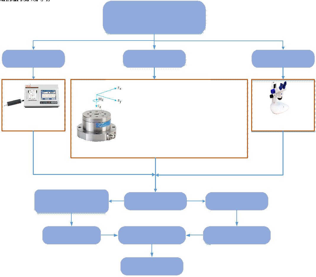
Figure 1 Diagram of experimental design
The Kistler piezoelectric dynamometer type 9272 was used to estimate the three orthogonal components of the end-milling cutting forces: cutting force in the x direction (Fx), cutting force in y direction (Fy), and cutting force in the z-direction/thrust (Fz). Four piezoelectric force sensors on the dynamometer produce voltage outputs that vary directly with the load acting on the sensor. The voltage is then amplified using a Kistler charge amplifier 5070 A. A data acquisition system (Kistler 5097 A) is then employed for connecting and controlling the charge amplifiers and signal conditioners. The signal is then calibrated using Kistler Dyno Ware software via the RS-232 serial interface. The resultant of three measured forces or CF calculated by using Equation(1) (Soepangkat et al., 2019):
SR measurements were performed by using Mitutoyo Surftest SJ 310. Since the surface roughness values are in the range of 1-3 µm, based on the standard EN ISO 4288, the recommended cut-off wavelength (?c) range is 0.8 mm and 2.5 mm, and the evaluation length (ln) consists of 5 sampling lengths (4 and 10 mm). An example of a macro imaged slot is depicted in Figure 2. The width of the slot is denoted by the letter W (equal to the diameter of end-milling), where the maximum damaged width or delamination factor, as assessed by using CAD, is Wmax. The delamination factor for each slot can be calculated using equation 2 (Jenarthanan et al., 2017; Kiliçkap et al., 2015; Çelik et al., 2014; Erkan et al., 2013):
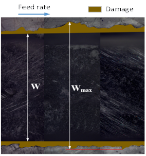
Figure 2 The macro imaged slot
Optimization Process
Back Propagation Neural Network (BPNN)
A BPNN model possesses input, hidden, and output layers, each with several neurons connected. The bias and weight of each neuron in each layer represent the link that connects the input and output layers. During the BPNN model training, the bias and weight for each neuron will be adjusted utilizing an error function to lower the error gradually. The optimal network design that yields the minimum mean squared error (MSE), response prediction, and goal function is the result of developing the BPNN model. The following are the steps for creating a BPNN model (Wang et al., 2019; Soepangkat et al., 2019): (a) Selecting the appropriate training function and conducting training, testing, and validation, (b) Creating the BPNN network design by determining the parameters of modelling which include variations of hidden layers and neurons in the hidden layers, stopping criteria or maximum iterations, learning rate, and activation functions for hidden and output layers, (c) Comparing the predicted results from BPNN output with the experimental results, (d) Collecting the BPNN pattern and objective function.
Simulated Annealing Algorithm (SAA)
SAA is considered a stochastic optimization tool for solving nonlinear programming (NLP) issues. The primary concept behind SAA is to produce random locations to elude becoming stuck in a local minimum. According to (Dowsland and Thompson, 2012), the SAA can be summarized as follows:
Choosing a new solution (s), initial solution (s0), initial temperature (T0), maximum iteration, and maximum sub-iteration, the fitness function of the new solution (f(s)), and fitness function of initial solution (f(s0)).
Examining the fitness function difference () using the following equation.
Generate random value (x) in the limits (0,1)
If x < exp-T0 , a new solution (s) is used to replace the initial solution (s0), and go to step 5.
If x > exp-T0 , go to step 5.
Lowering the temperature and ensuring that the termination requirement has been met. The cooling schedule for lowering temperature was computed using equation (4)
where Tk is the latest temperature, To is an initial temperature, and c and k are constants.
Repeating steps 2 to 5 until a maximum number of iterations until the SAA is terminated.
Firefly algorithm (FA)
Firefly algorithm (FA) was built on the behavior of a swarm of fireflies. The intensity of fireflies' light is linked to their attraction parameter. The Euclidean distance formula can be used to calculate the range between the fireflies. The current location of the firefly (ith), eagerness to approach other appealing fireflies (jth), and product of randomization constraint (?) and a random number (?i) are factors considered in updating the firefly position. The FA can be proceduralized as follows (Fister et al., 2013):
Initializing the random locations of the firefly inside the variables' border after defining the objective function.
Assessing the intensity of light (or fitness value) for all fireflies.
Choosing the best firefly depends on the light intensity value.
Calculating the distance between the best and other fireflies (r). Further, equation (5) can be used to calculate the distance between two fireflies i and j:
The kth component of the spatial coordinate xi of ith is xi,k.
Changing the location of the fireflies. The motion of a firefly attracted by another firefly can be determined by using the following equation:
where () is the scaling parameter that can be computed using equation (7), where ? is a randomness reduction parameter:
Furthermore, the attractiveness parameter () is then calculated using the following formulation:
where o is the initial attractiveness parameter, and is the media light absorption coefficient, and r is the range between two fireflies.
Analyzing the intensity rate, fireflies' intensities, and location of the fireflies.
Choosing the most appropriate firefly for the current iteration. The overall process is then repeated until the FA's stopping criteria are satisfied.
Genetic Algorithm (GA)
The genetic algorithm (GA) is a commonly used population-based metaheuristic or soft computing method for solving optimization problems in mathematics, engineering, and other subjects (Sekulic et al., 2018; Mahesh et al., 2015). The steps of a generic GA are as follows (Soepangkat et al., 2019; Sekulic et al., 2018; Mahesh et al., 2015): generating N solutions at random to form the first population, calculating the solution's fitness values, selection, crossover, and mutation.
Findings
Figure 3 represents the experimental process and response measurement. As a result of the combination of n, Vf, and d, Table 2 illustrates the measured CF, SR, and DF successively. This table reveals that CF, SR, and DF values trace a steady path in a reasonable interval of end-milling process parameters.
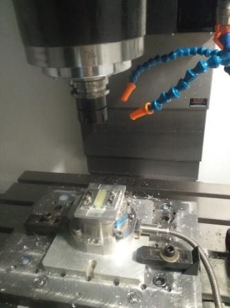
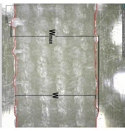
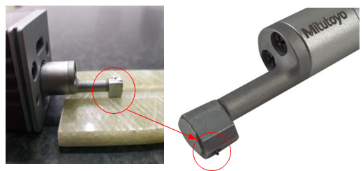
Figure 3 Response Measurement for (a) Cutting force, (b) Delamination, (c) Surface roughness.
BPNN Model Development
The first stage in modelling is to normalize the experimental data to make sure that the interval value is between -1 and 1 using a normalization method of MATLAB 2022b. The best BPNN network structure had an MSE score of 0.17457 with an architectural network option was 3 - 8 - 8 - 8 - 3, where the predicted cutting force, surface roughness, and delamination factor all had average errors of 2.806%, 4.311%, and 0.026%, respectively, as shown in Table 2. An error between the experiment and prediction is calculated using the following equation:
Table 2 The measured CF, SR, and DF using the combination of n, Vf, and d.
Table 2 The measured CF, SR, and DF using the combination of n, Vf, and d (Cont.)
Table 2 The measured CF, SR, and DF using the combination of n, Vf, and d. (cont.)
3.3. Fitness Function
Fitness function is generated using three objectives, i.e., CF, SR, and DF, as shown in the following equation:
Where Obj1 is an objective function of CF, Obj2 is an objective function of SR, and Obj3 is an objective function of DF.
3.4. Optimization of Multi-Performance Using FA, GA, SAA, GA-SAA
Parameters used in BPPN modelling and optimization methods (GA, FA, and SAA) can be seen in Table 3 and Table 4.
Table 5 compares optimization results using FA, GA, SAA, and GA- SAA. Again, the combination of GA and SAA produced the lowest fitness value compared with the other optimization methods. As a result, n, Vf, and d for the end-milling process of GFRP composites are 4357.65 rpm, 563.57 mm/min, and 1.26 mm, respectively.
Table 3 Parameters utilized in BPNN modelling
Table 4 Parameters utilized in Optimization methods (GA, FA, and SAA)
Table 5 The comparison of optimization results using FA, GA, SAA, and GA-SAA
3.5. Effects of End-Milling Process Parameters on Responses
ANOVA was utilized to calculate the percent contribution of end-milling parameters on the total variance of the CF, SR, and DF. Table 6 shows the percent contribution of each end-milling parameter to the total variance. Regarding all three responses, Vf was the highest contributor to the total variance, followed by d and n as the second and third contributors to the total variance of CF. Meanwhile, the second and third contributors to the total variance of SR and DF were n and d. In addition, several researchers obtained the same results for CF (Soepangkat et al., 2019; Sekulic et al., 2018), SR (Raj et al., 2020; Jenarthanan et al., 2017; Rajesh Mathivanan et al., 2016; Kiliçkap et al., 2015; Mahesh et al., 2015). Furthermore, the effects of the end-milling parameters on CF, SR, and DF were examined using response graphs presented in Figures 4, 5, and 6.
Figure 4 depicts the effects of the end-milling parameters on CF. As the Vf and d rise, the CF increases, and while n increases, the CF reduces. It is easy to see how raising n reduces the CF. This phenomenon occurs because when n increases, the friction force on the cutting surface increases, resulting in the temperature elevation on the cutting surface. Since the thermal conductivity of glass fiber and epoxy resin is low, the heat produced on the cutting surface cannot be dismissed easily.
Table 6 Percent contribution of end-milling parameters for each response.
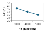
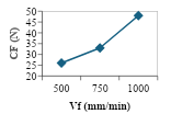
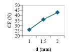
Figure 4 The end-milling parameters' effects on Cutting Force (CF)
Further, with the concentration of heat in the cutting area, the matrix around this area becomes softer, and CF decreases. The factor that has the most significant impact on CF is feed speed. A faster feed speed increases the undeformed chip cross-sectional area (Azmi et al., 2013). In addition, the cut depth considerably impacts the response to the CF. The increase in d would increase the cross-sectional area and the number of fibers cut, increasing CF. (Jenarthanan et al., 2017; Rajesh Mathivanan et al., 2016; Çelik et al., 2014) came up with the same findings.
Figure 5 depicts the end-milling parameters' effects on SR. As n is increased, SR decreases. This phenomenon happens because increasing n lowers the distortion of the tool-chip interface, resulting in a smoother surface. The high value of n should not be used; however, because GFRP is an abrasive material, it can cause premature tool wear. Figure 11 further illustrates that increasing Vf appears to enhance the SR. Increasing Vf causes the composite material strain rate to grow, yielding significant fissures in the epoxy and glass fiber (Azmi et al., 2013). The escalation in SR produced by increasing Vf is consistent with the theoretical surface roughness equation (Stephenson and Agapiou, 2016). SR decreases as n increases, but SR appears to rise with d increases; however, the effect is minor. (Raj et al., 2020; Stephenson and Agapiou, 2016) also indicated similar findings.
The effect of process parameters on DF is shown in Figure 6. As n and Vf rise, DF increases considerably. This could be due to increased speeds, which raise the cutting surface's friction force and cause the cutting surface temperature to rise. Since the thermal conductivity of both glass fiber and epoxy resin is low, the heat resulting on the cutting surface cannot be dismissed easily. The intense heat in the cutting area weakens the link between the matrix and the fibers, resulting in delamination. The faster the Vf, the more cutting force is generated, resulting in more delamination. Although just slightly, increasing the depth of cut increases DF. These findings were comparable to those of (Raj et al., 2020; Kiliçkap et al., 2015; Erkan et al., 2013).
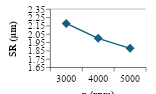
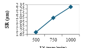
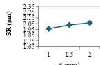
Figure 5 The end-milling parameters' effects on Surface Roughness (SR)


Figure 6 The end-milling parameters' effects on Delamination Factor (DF)
Figure 7 illustrates the delamination on one side of the cut slot when the cut width is greater than the slot width (equal to the end-milling diameter). It is shown that the fiber has been cut, and the matrix/resin part has been peeled off or crushed.
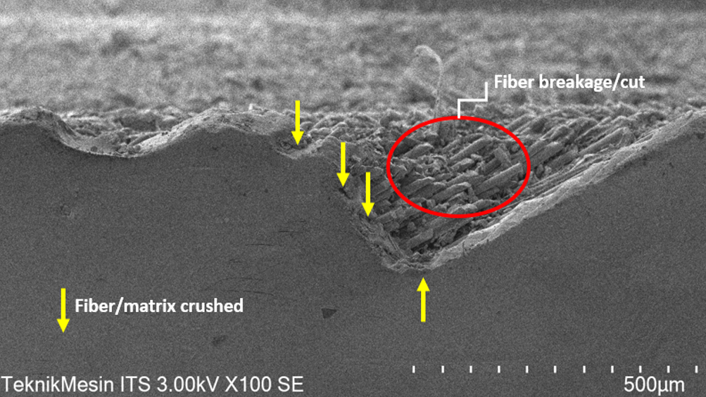
Figure 7 A SEM image illustrates the delamination on one side of the cut slot
3.6. Confirmation Experiment
The minimal CF, SR, and DF were reached by setting n, Vf, and d to 4357.65 rpm, 563.57 mm/min, and 1.26 mm, respectively, using the BPNN GA-SAA method to solve the multi-response optimization. The confirmation experiment is then repeated five times with the best end-milling parameter settings, as shown in Table 7. It has been observed that the deviation between the predicted outcomes of the BPNN-GA-SAA model and the actual results of the confirmation experiment does not exceed 5% for all responses. This suggests that the predicted response of the end-milling process is in close agreement with the actual experimental results.
Table 7 Comparison between BPNN-GA-SAA prediction and confirmation experiments.
This study used the integration of BPNN, FA, GA, SAA, and GA-SAA to predict the best combination of end-milling parameters of GFRP composites. The cutting force, surface roughness, and delamination factor are end-milling parameters were predicted using BPNN, with an MSE value is 0.17457. Since the resulting average error is less than 5%, BPNN has effectively forecasted the minimum value of cutting force, surface roughness, and delamination factor after being appropriately applied. SAA was found as the fastest method to solve the optimization problem. However, GA-SAA was the best method to predict the best optimization result. The findings of using a hybrid BPNN-GA-SAA for optimization show that by arranging the rotational speed, feed speed, and axial depth of cut to 4357.65 rpm, 563.57 mm/min, and 1.26 mm, respectively, the minimum values of cutting force, surface roughness, and delamination factor can be obtained simultaneously. Furthermore, based on the ANOVA, feed speed contributes the most to the total variance of cutting force, surface roughness, and delamination factor. The graphical analysis confirms that the three responses increased considerably with increasing feed speed compared to the increasing axial depth of cut. Meanwhile, increasing spindle speed would decrease the cutting force and surface roughness but increase delamination. The SEM analysis indicates that delamination mainly consists of fiber cuts and the peeling or crushing of the matrix/resin. The prediction performance of BPNN can be improved by increasing experimental data sets, for example, using finite element methods to reduce experimental costs.
The authors would like to thank DRPM, Institut Teknologi Sepuluh Nopember, Surabaya, Indonesia, for providing Research Grant number 860/PKS/ITS/2020
Author Contributions
Mohammad Khoirul Effendi conceptualized the study and developed the hybrid optimization methods. Rachmadi Norcahyo conducted experiments and collected data. Mohammad Khoirul Effendi and Bobby O. P. Soepangkat performed data analysis and visualization. Bobby O. P. Soepangkat and Dinny Harnany. wrote the original draft of the manuscript.
Conflict of Interest
The authors declare no conflicts of interest
Azmi, AI, Lin, RJT & Bhattacharyya, D 2013, ‘Machinability study of glass fibre-reinforced polymer composites during end milling’, International Journal of Advanced Manufacturing Technology, vol. 64, pp. 247–261, https://doi.org/10.1007/s00170-012-4006-6
Becker, F, Hopmann, C, Italiano, F, Girelli, A & Spagnuolo, S 2019, ‘Fatigue testing of GFRP materials for the application in automotive leaf springs’, Procedia Structural Integrity, Fatigue Design 2019, International Conference on Fatigue Design, 8th Edition, vol. 19, pp. 645–654, https://doi.org/10.1016/j.prostr.2019.12.070
Bharathi Raja, S, Srinivas Pramod, CV, Vamshee Krishna, K, Ragunathan, A & Vinesh, S 2015, ‘Optimization of electrical discharge machining parameters on hardened die steel using Firefly Algorithm’, Engineering Computations, vol. 31, pp. 1–9, https://doi.org/10.1007/s00366-013-0320-3
Budiyantoro, C, Rochardjo, HSB, Wicaksono, SE, Ad, MA, Saputra, IN & Alif, R 2024, ‘Impact and Tensile Properties of Injection-Molded Glass Fiber Reinforced Polyamide 6 –Processing temperature and pressure optimization’, International Journal of Technology, vol. 15(3), pp. 597–607, https://doi.org/10.14716/ijtech.v15i3.5404
Caratelli, A, Meda, A, Rinaldi, Z, Spagnuolo, S & Maddaluno, G 2017, ‘Optimization of GFRP reinforcement in precast segments for metro tunnel lining’, Composite Structures, vol. 181, pp. 336–346, https://doi.org/10.1016/j.compstruct.2017.08.083
Çelik, YH, K?l?çkap, E & Yard?meden, A 2014, ‘Estimate of cutting forces and surface roughness in end milling of glass fibre reinforced plastic composites using fuzzy logic system’, Science and Engineering of Composites Materials, vol. 21, pp. 435–443, https://doi.org/10.1515/secm-2013-0129
Dawood, LL & AlAmeen, ES 2024, ‘Influence of infill patterns and densities on the fatigue performance and fracture behavior of 3D-printed carbon fiber-reinforced PLA composites’, AIMS Materials Science, vol. 11, pp. 833–857, https://doi.org/10.3934/matersci.2024041
Dowsland, KA & Thompson, JM 2012, ‘Simulated annealing’, in Rozenberg, G, Bäck, T, Kok, JN (Eds.), Handbook of Natural Computing, Springer, Berlin, Heidelberg, pp. 1623–1655, https://doi.org/10.1007/978-3-540-92910-9_49
Erkan, Ö, I??k, B, Çiçek, A & Kara, F 2013, ‘Prediction of damage factor in end milling of glass fibre reinforced plastic composites using artificial neural network’, Applied Composites Materials, vol. 20, pp. 517–536, https://doi.org/10.1007/s10443-012-9286-3
Fister, I, Fister, I, Yang, X-S & Brest, J 2013, ‘A comprehensive review of firefly algorithms’, Swarm and Evolutionary Computation, vol. 13, pp. 34–46, https://doi.org/10.1016/j.swevo.2013.06.001
Gautam, GD & Mishra, DR 2019, ‘Firefly algorithm based optimization of kerf quality characteristics in pulsed Nd:YAG laser cutting of basalt fiber reinforced composite’, Composites Part B: Engineering, vol. 176, p. 107340, https://doi.org/10.1016/j.compositesb.2019.107340
Giammaria, V, Capretti, M, Del Bianco, G, Boria, S & Santulli, C 2024, ‘Application of poly(lactic acid) composites in the automotive sector: a critical review’, Polymers, vol. 16, p. 3059, https://doi.org/10.3390/polym16213059
Jenarthanan, MP, Gokulakrishnan, R, Jagannaath, B & Raj, PG 2017, ‘Multi-objective optimization in end milling of GFRP composites using Taguchi techniques with principal component analysis’, Multidisciplinary Modeling in Materials and Structures, vol. 13, pp. 58–70, https://doi.org/10.1108/MMMS-02-2016-0007
Kiliçkap, E, Yardimeden, A & Çelik, YH 2015, ‘Investigation of experimental study of end milling of CFRP composite’, Science and Engineering of Composites Materials, vol. 22, pp. 89–95, https://doi.org/10.1515/secm-2013-0143
Liu, Z, Li, X, Wu, D, Qian, Z, Feng, P & Rong, Y 2019, ‘The development of a hybrid firefly algorithm for multi-pass grinding process optimization’, Journal of Intelligent Manufacturing, vol. 30, pp. 2457–2472, https://doi.org/10.1007/s10845-018-1405-z
Lobato, FS, Sousa, MN, Silva, MA & Machado, AR 2014, ‘Multi-objective optimization and bio-inspired methods applied to machinability of stainless steel’, Applied Soft Computing, vol. 22, pp. 261–271, https://doi.org/10.1016/j.asoc.2014.05.004
Lololau, A, Soemardi, TP, Purnama, H & Polit, O 2021, ‘Composite Multiaxial Mechanics: Laminate Design Optimization of Taper-Less Wind Turbine Blades with Ramie Fiber-Reinforced Polylactic Acid’, International Journal of Technology, vol. 12(6), pp. 1273–1287, https://doi.org/10.14716/ijtech.v12i6.5199
Mahesh, G, Muthu, S & Devadasan, SR 2015, ‘Prediction of surface roughness of end milling operation using genetic algorithm’, International Journal of Advanced Manufacturing Technology, vol. 77, pp. 369–381, https://doi.org/10.1007/s00170-014-6425-z
Majumder, A 2015, ‘Comparative study of three evolutionary algorithms coupled with neural network model for optimization of electric discharge machining process parameters’, In: Proceedings of the Institution of Mechanical Engineers, Part B: Journal of Engineering Manufacture, vol. 229, pp. 1504–1516, https://doi.org/10.1177/0954405414538960
Mohammadi, H, Ahmad, Z, Mazlan, SA, Faizal Johari, MA, Siebert, G, Petr?, M & Rahimian Koloor, SS 2023, ‘Lightweight glass fiber-reinforced polymer composite for automotive bumper applications: a review’, Polymers, vol. 15, article 193, https://doi.org/10.3390/polym15010193
Morampudi, P, Namala, KK, Gajjela, YK, Barath, M & Prudhvi, G 2021, ‘Review on glass fiber reinforced polymer composites’, Materials Today Proceedings, 1st International Conference on Energy, Material Sciences and Mechanical Engineering, vol. 43, pp. 314–319, https://doi.org/10.1016/j.matpr.2020.11.669
Prasanth, ISNVR, Ravishankar, DV, Hussain, MM, Badiganti, CM, Sharma, VK & Pathak, S 2018, ‘Investigations on performance characteristics of GFRP composites in milling’, International Journal of Advanced Manufacturing Technology, vol. 99, pp. 1351–1360, https://doi.org/10.1007/s00170-018-2544-2
Raj, PP, Pazhanivel, K & Ganesh, NS 2020, ‘Measurement of delamination and tool wear with sensors in end-milling using solid and carbide-tipped K10 end mills’, International Journal of Materials and Product Technology, vol. 61, pp. 262–277, https://doi.org/10.1504/IJMPT.2020.113191
Rajesh Mathivanan, N, Mahesh, BS & Anup Shetty, H 2016, ‘An experimental investigation on the process parameters influencing machining forces during milling of carbon and glass fiber laminates’, Measurement, vol. 91, pp. 39–45, https://doi.org/10.1016/j.measurement.2016.04.077
S?ftoiu, GV, Constantin, C, Nicoar?, AI, Pelin, G, Ficai, D & Ficai, A 2024, ‘Glass fibre-reinforced composite materials used in the aeronautical transport sector: a critical circular economy point of view’, Sustainability, vol. 16, p. 4632, https://doi.org/10.3390/su16114632
Sekulic, M, Pejic, V, Brezocnik, M, Gostimirovic, M & Hadzistevic, M 2018, ‘Prediction of surface roughness in the ball-end milling process using response surface methodology, genetic algorithms, and grey wolf optimizer algorithm’, Advances in Production Engineering & Management, vol. 13, pp. 18–30, https://doi.org/10.14743/apem2018.1.270
Senthilkumar, N, Tamizharasan, T & Gobikannan, S 2014, ‘Application of response surface methodology and firefly algorithm for optimizing multiple responses in turning AISI 1045 steel’, Arabian Journal for Science and Engineering, vol. 39, pp. 8015–8030, https://doi.org/10.1007/s13369-014-1320-3
Seo, T, Song, B, Seo, K, Cho, J & Yoon, G 2011, ‘A study of optimization of machining conditions in micro end-milling by using response surface design’, International Journal of Technology, vol. 2(3), pp. 248–256, https://doi.org/10.14716/ijtech.v2i3.74
Shivanagere, A, Sharma, SK & Goyal, P 2018, ‘Modelling of glass fibre reinforced polymer (gfrp) for aerospace applications’, Journal of Engineering Science and Technology, vol. 13, pp. 3710–3728
Shukla, R & Singh, D 2017, ‘Experimentation investigation of abrasive water jet machining parameters using Taguchi and Evolutionary optimization techniques’, Swarm and Evolutionary Computation, vol. 32, pp. 167–183, https://doi.org/10.1016/j.swevo.2016.07.002
Soepangkat, BO, Pramoedyo, NO, Norcahyo, R, Pramujati, B & Wahid, MA 2019, ‘Multi-objective optimization in face milling process with cryogenic cooling using grey fuzzy analysis and BPNN-GA methods’, Engineering Computations, vol. 36, pp. 1542–1565, https://doi.org/10.1108/EC-06-2018-0251
Soepangkat, BO, Pramujati, B, Effendi, MK, Norcahyo, R & Mufarrih, AM 2019, ‘Multi-objective optimization in drilling kevlar fiber reinforced polymer using grey fuzzy analysis and backpropagation neural network–genetic algorithm (BPNN–GA) approaches’, International Journal of Precision Engineering and Manufacturing, vol. 20, pp. 593–607, https://doi.org/10.1007/s12541-019-00017-z
Stephenson, DA & Agapiou, JS 2016, Metal cutting theory and practice, Third edition, Metal Cutting Theory and Practice, Third Edition
Sulaiman, S, Alajmi, MS, Wan Isahak, WN, Yusuf, M & Sayuti, M 2022, ‘Dry milling machining: optimization of cutting parameters affecting surface roughness of aluminum 6061 using the taguchi method’, International Journal of Technology, vol. 13(1), pp. 58–68, https://doi.org/10.14716/ijtech.v13i1.4208
Thakur, RK, Sharma, D & Singh, KK 2019, ‘Optimization of surface roughness and delamination factor in end milling of graphene modified GFRP using response surface methodology’, Materials Today Proceedings, 1st International Conference on Manufacturing, Material Science and Engineering, vol. 19, pp. 133–139, https://doi.org/10.1016/j.matpr.2019.06.153
Tudjono, S, Lie, HA & Gan, BS 2018, ‘An integrated system for enhancing flexural members’ capacity via combinations of the fiber reinforced plastic use, retrofitting, and surface treatment techniques’, International Journal of Technology, vol. 9, no. 1, pp. 5–15, https://doi.org/10.14716/ijtech.v9i1.298
Wang, A, Tang, X, Zeng, Y, Zou, L, Bai, F & Chen, C 2024, ‘Carbon fiber-reinforced PLA composite for fused deposition modeling 3D printing’, Polymers, vol. 16, p. 2135, https://doi.org/10.3390/polym16152135
Weichert, D, Link, P, Stoll, A, Rüping, S, Ihlenfeldt, S & Wrobel, S 2019, ‘A review of machine learning for the optimization of production processes’, International Journal of Advanced Manufacturing Technology, vol. 104, pp. 1889–1902, https://doi.org/10.1007/s00170-019-03988-5